Case study · river flooding in all 260 districts of Ghana

Ghana flood risk: where to act first

A national flood risk screening is only useful if it changes where a country acts first, and for whom. I screened all 260 districts for damage and for people exposed, tested which priorities hold under uncertainty, presented the results for discussion with the World Bank and am now sharing them with its Accra-based team.

Role
Independent consultant (sole analyst)
Period
2025–26
Estimated value
est. US$90k (US$155k with the coastal work)
Status
Complete

Independent consultancy; the river work was also my Oxford MSc dissertation. Values are estimates.

Screening tier: it decides where to look next, not what to build

  • 13 Act
  • 13 Investigate
  • 234 Monitor

All 260 districts. Act: in the national top 20 for modelled damage in all nine combinations; Investigate: in some; Monitor: in none, which does not mean safe. Not an official priority list.

modelled residential flood damage a year (median; about US$413m)
GHS5.19bn
of that modelled annual damage falls in 20 of the 260 districts
86.8%
people inside the modelled 1-in-100-year flood extent, including about 421,700 children
1.18million
district-level damage calculations in a Monte Carlo (Latin hypercube) analysis
11.7million

Before the flood: understanding risk

Where river flood risk concentrates, and which priorities hold

The map shows which districts to look at first. Act districts stay in the national top 20 for flood damage whatever the assumptions (all nine combinations of flood extent and damage curve); Investigate districts in some; Monitor districts in none.

Fig. 1

Ghana’s 260 districts by priority class, modelled annual damage or people exposed

Hover, tab to or choose a district. Monitor does not mean safe; this is not an official priority list.

Sources

Independent consultancy (2025–26); the river work was also my Oxford MSc dissertation. Hazard: JRC Global River Flood Hazard Maps v2 (CC BY 4.0). Buildings: Google Open Buildings. People: WorldPop (CC BY 4.0). Boundaries: OCHA/HDX COD-AB (GSS). Not official estimates of the Government of Ghana or the World Bank.

Why a short list matters

Twenty districts, mostly on the lower Volta and the fringe of Greater Accra, hold 86.8% of the modelled annual damage. The top five alone hold 49%. That concentration is what makes a national screen useful: it narrows 260 local authorities to a shortlist where detailed appraisal is worth paying for.

The colouring answers a second question. A district that tops the list under one set of assumptions but drops out under another is a weaker basis for spending than one that stays near the top whatever the assumptions. The 13 Act districts are robust in that sense.

The method in ten steps, from open data to a decision rule

How the analysis was built, one stage at a time, from where floods reach to which districts come first. I built every stage in Python, GDAL and QGIS on a national 90 m grid; open a stage for its inputs, code and limits.

Fig. 2 · Process map

Ten stages of the national screening, from open data to a decision rule

Scroll through the ten stages, or choose one.Choose a stage to show it on the map. The map shows what each stage adds.

Step 1 of 10 · River flood depths

Flood hazard

Global river flood-depth maps from the EU Joint Research Centre give modelled water depth for floods from 1-in-10 to 1-in-500 years on a common 90 m grid across Ghana. A 1-in-100-year flood has a 1% chance of happening in any year.

5flood return periods, 1-in-10 to 1-in-500 years

Inputs, process, outputs and limitation

Inputs

  • JRC Global River Flood Hazard Maps v2 (Dottori et al., 2024): ~90 m depth rasters produced by JRC with LISFLOOD hydrology and LISFLOOD-FP inundation; RP10, 50, 100, 200, 500 used
  • Ghana district boundaries (admin level 2, 260 polygons)

Process, as coded

Tiles mosaicked and reprojected to UTM 30N (EPSG:32630) with GDAL; read with rasterio (read_raster(), nodata set to 0). Alternatives compared: WRI Aqueduct (~900 m) and UNEP/CIMA GIRI (90 m).

Outputs

Five aligned depth rasters (jrc_rp{RP}_mosaic_epsg32630.tif), each 7,939 × 5,502 cells at 90 m.

Limitation

Published JRC outputs were used as given, with no local hydraulic model, so channels, defences and urban drainage are not represented. River flooding only.
Step 2 of 10 · White Volta 2020 test

Hazard check

The modelled 10-year flood extent was compared with satellite-observed flooding from the September 2020 White Volta flood in five 20 × 20 km test areas.

0.58mean Critical Success Index (range 0.43–0.71)

Inputs, process, outputs and limitation

Inputs

  • Sentinel-1-derived flood extent, September 2020, 20 m, aggregated to flooded fraction on the 90 m grid (flooded if ≥10% of the cell)
  • JRC RP10 depth raster

Process, as coded

Modelled = depth > 0; observed = fraction ≥ 0.10. Area-of-interest centres converted from WGS84 with pyproj; ±111-cell (20 km) windows. Critical Success Index = overlap ÷ union. Directed nearest-flooded-pixel distances with scipy distance_transform_edt (0.09 km per cell); 90th percentile of misses and excess (np.percentile).

Outputs

CSI and P90 miss/excess distances per test area. These set the spatial stress tests: contract the flood edge by 2 cells, expand by 1 cell.

Limitation

One event whose size need not match a 10-year flood, and satellites can miss short-lived flooding. In one test area misses reached 2.8 km, so no single boundary offset fits everywhere.

Step 3 of 10 · Who lives there

People

2026 gridded population estimates for all residents, children (0–14) and older people (65+) were aligned to the 90 m grid. Census shares added people with functional difficulties (disability).

1.18 millionpeople inside the modelled 1-in-100-year flood extent

Inputs, process, outputs and limitation

Inputs

  • WorldPop Global2 2026 estimates (~100 m): total, ages 0–14, 65+
  • Ghana Statistical Service 2021 Population and Housing Census: district age and functional-difficulty tables
  • District boundaries (260)

Process, as coded

Census tables filtered (All Locality Types, Both sexes); district shares computed; names harmonised to 260 boundary polygons; shares rasterised (rasterio.features.rasterize) and multiplied by population; raster sums checked for conservation. Exposure: population in cells with modelled flood depth, summed by district.

Outputs

90 m rasters of population, children, older people and people with functional difficulty; exposure by district and return period.

Limitation

Disability shares are spread evenly within each district, and the uncertainty runs rescale population without moving anyone, so errors in where people live are untested.

Step 4 of 10 · What is exposed

Buildings

About 13 million building footprints detected from satellite imagery were converted to floor area on the 90 m grid.

~13 millionbuilding footprints mapped (1,080.6 million m²)

Inputs, process, outputs and limitation

Inputs

  • Google Open Buildings v3 footprints (confidence ≥ 0.65)
  • 2021 census storey shares: 95.76% one level, 3.57% two, 0.48% three

Process, as coded

Footprints rasterised to footprint area per 90 m cell. Floor area = footprint × storey factor (sampled 1.01–1.10, mode 1.04).

Outputs

National footprint-area raster (1,080.6 million m²) and floor area.

Limitation

Every detected building is treated as residential and mostly single-storey. Detection errors are covered only by a national ±15% multiplier.

Step 5 of 10 · What it is worth

Asset value

A replacement-cost map (GHS per m²) was built from night-time lights, calibrated at ten Ghanaian neighbourhoods and checked against census poverty data.

ρ = 0.83rank correlation with census welfare, 260 districts (p < 0.001)

Inputs, process, outputs and limitation

Inputs

  • VIIRS night-time lights (2024 annual average, ~500 m), 2 km neighbourhood median
  • 10 calibration neighbourhoods (GHS 1,250–5,500 per m²) from construction-cost guides, imagery and listings; UN-Habitat 2011 low-cost anchor
  • GSS district multidimensional-poverty incidence

Process, as coded

Cost = clip(−744.08 + 1,206.68 × ln(1 + radiance), 1,250, 7,000) GHS/m² (log form chosen over linear and square-root). Contents = 0.5 × structure. Value = floor area × cost × (1 + contents). District mean cost vs welfare (100 − poverty incidence) tested with Spearman correlation (scipy spearmanr).

Outputs

90 m replacement-cost raster; exposed residential asset value. National median stock about GHS 3.84 trillion.

Limitation

Calibration costs are judgement-based. The welfare check confirms ranking, not monetary accuracy. The 0.5 contents ratio is well above the GEM model’s ~0.19.

Step 6 of 10 · How much is damaged

Vulnerability

Three depth–damage curves convert flood depth into the share of building and contents value lost. They are tested as alternative models, not averaged.

10%, 38%, 59%damage at 1 m depth under the three curves (widest disagreement)

Inputs, process, outputs and limitation

Inputs

  • JRC Africa residential (Huizinga et al., 2017), reference
  • Accra-selected Sri Lanka transfer (World Bank, 2020)
  • Ouagadougou semi-concrete (Karambiri et al., 2015)

Process, as coded

13-point curves (0–6 m in 0.5 m steps), linear interpolation per cell (np.interp). The same fraction is applied to structure and contents.

Outputs

Damage fraction for every cell, return period, flood extent and curve.

Limitation

No curve is derived from Ghanaian damage records. Flooded building cells are deep (median 2.9 m at RP10), so results lean on the upper part of the curves at coarse 90 m depth.

Step 7 of 10 · Expected annual damage

Damage and annual risk

Losses for each flood size were summed by district and turned into expected annual damage (EAD): the average loss to expect each year, with each flood weighted by its chance of happening.

GHS 5.19bn / yrnational median EAD (≈US$413m); 86.8% in 20 districts

Inputs, process, outputs and limitation

Inputs

  • Exposed value and damage fractions (stages 4–6)
  • District grid (district_id_90m)

Process, as coded

Base damage = Σ footprint area × cost × damage fraction per district. Probabilities: RP10 0.10, RP50 0.02, RP100 0.01, RP200 0.005, RP500 0.002. EAD = trapezoidal integral of loss over p = 0.10 to 0.002 (np.trapezoid).

Outputs

District and national losses per flood; EAD₁₀–₅₀₀ by district.

Limitation

Covers only 10- to 500-year floods; more frequent and rarer events are excluded. Counts homes and contents only, not infrastructure, farms or businesses.

Step 8 of 10 · Monte Carlo (Latin hypercube)

Uncertainty ensemble

Monte Carlo (Latin hypercube) sampling, a way of drawing random but evenly spread values, varied seven uncertain inputs 1,000 times. Each sample was run under three flood extents and three damage curves.

2.5×national EAD across flood extents: GHS 2.93bn (contracted) to 7.33bn (expanded)

Inputs, process, outputs and limitation

Inputs

  • Triangular ranges for population, child and older-person shares, building count, storeys, replacement value and contents
  • Three flood-extent states and three damage curves

Process, as coded

scipy qmc.LatinHypercube (seed 42; 3 population and 4 economic dimensions), mapped to triangular distributions (scipy triang.ppf). Damage = base damage × building × storey × value multipliers × (1 + contents ratio). P5 / median / P95 summaries; Spearman sensitivity of national EAD to each input.

Outputs

11.7 million district-level damage calculations; 2.34 million district EAD values; 15,000 national population-exposure runs.

Limitation

Ranges are assumed, not fitted to data. Economic multipliers apply nationally, so they change totals but cannot reorder districts. The nine combinations carry no probabilities.

Step 9 of 10 · Against reported impacts

Consequence check

Modelled people and buildings in the observed 2020 White Volta flood footprint were compared with disaster-agency (NADMO) reports, and national losses with earlier assessments.

84%6,371 people modelled vs 7,561 reported affected

Inputs, process, outputs and limitation

Inputs

  • Observed 2020 flooded fraction (739.7 km²)
  • NADMO-reported impacts (via FloodList, 2020)
  • UNDRR/CIMA 2019 Ghana risk profile; Croitoru et al. (2019) Côte d’Ivoire and Senegal

Process, as coded

People affected = Σ population × observed flooded fraction. Buildings intersecting the footprint counted at baseline and after a one-cell expansion. Event loss uses JRC RP10 depth as a depth analogue. Loss-to-stock and GDP-scaled regional comparisons.

Outputs

Plausibility checks on people, buildings and national loss scale.

Limitation

Modelled buildings rise from 474 to 3,073 after a one-cell shift, against 1,596 reported damaged houses: results hinge on where settlements sit at the flood edge. No observed monetary losses exist to validate damage.

Step 10 of 10 · Which priorities hold

Decision: Act / Investigate / Monitor

Districts were ranked by expected annual damage in each of the nine combinations. Those in the national top 20 every time are “Act”, some of the time “Investigate”, and never “Monitor”.

13, 13, 234Act, Investigate, Monitor districts

Inputs, process, outputs and limitation

Inputs

  • District EAD for 1,000 samples × 9 combinations

Process, as coded

Rank within each sample and combination (pandas rank, highest damage first; tied districts take the best rank). Top-20 frequency = share of samples ranked ≤ 20. Act if min frequency ≥ 0.80 across combinations; Investigate if max ≥ 0.20; otherwise Monitor. Top-10 and Top-30 run as sensitivity checks. Level-2 screen combines EAD, top-20 boundary crossing and loss range across flood extents.

Outputs

National Act–Investigate–Monitor map; Level-2 study candidates.

Limitation

Depends on an economic objective and an illustrative top-20 cut-off (top-10 gives 7 Act and 6 Investigate; top-30 gives 20 and 19). It shortlists where to appraise, not what to build.

Sources

Key numbers and limitations as reported in the dissertation. The map shows the Act, Investigate and Monitor classes, modelled damage and people; the test areas are the five used for the White Volta 2020 check.

Nuhu, H. (2026). National fluvial flood-risk assessment and priority stability under uncertainty in Ghana. MSc dissertation, School of Geography and the Environment, University of Oxford.

The core of the work, and what transfers to other countries

The uncertainty stage is the core of the work. Monte Carlo (Latin hypercube) analysis: 11.7 million district-level damage calculations. That is 1,000 samples of seven uncertain inputs, run under nine combinations of flood extent and damage curve, for 260 districts and five flood sizes.

Everything rests on open global datasets: JRC flood hazard, Google Open Buildings, WorldPop and VIIRS night lights. The same chain can be rebuilt for a data-scarce basin elsewhere, which is the transferable part. The Ghana numbers are not.

How a curve of flood losses becomes one annual figure

One number for flood risk: the damage to expect, on average, each year. It adds up each flood’s loss weighted by how likely that flood is in any year (the area under the loss curve), so frequent, moderate floods can matter more than rare, extreme ones.

Show the chart: damage per flood against its annual chance
Fig. 3

National damage per flood against its annual chance, and the annual damage beneath the curve

Median modelled residential damage including contents, baseline flood extent and JRC Africa damage curve. Hover or tab to a shaded band to see its share of the annual total.

Sources

Model estimate under stated assumptions; not an observed national loss.

What changes the answer, and by how much

How sure are these numbers? I re-ran the analysis 1,000 times, varying seven uncertain inputs, within each of nine combinations of flood extent and damage curve. Where the modelled flood edge sits matters far more than any economic assumption.

Show the chart: national annual damage under uncertainty
Fig. 4

National annual damage under uncertainty: three views of the same ensemble

(a) 1,000 samples for each flood extent, JRC Africa curve; (b) median and 5–95% range in each combination; (c) how strongly each input moves the total (Spearman rank correlation). A parameter range is not a confidence interval.

Sources

Contracted extent: flood edge pulled in 2 cells (180 m); expanded: pushed out 1 cell (90 m), set from the White Volta 2020 test distances.

The principle behind the test: robustness

The nine combinations are deliberately unweighted: there is no defensible basis for giving them probabilities. In that situation the World Bank’s guidance is that “accepting uncertainty mandates a focus on robustness” (Hallegatte et al., 2012), so the test is whether a district stays a priority under every combination, not what a single best estimate says.

“Base decisions on an understanding of risk and uncertainty.”

Golden Rule 3, Sayers et al. (2013), Box 2, p. 10, Flood Risk Management: A Strategic Approach, published by ADB

Plan and appraise

Which priorities hold under every assumption

The shortlist that survives the uncertainty: 13 districts stay in the national top 20 in all nine combinations, 13 more in some, and 234 in none. The cut-off itself is a policy choice to agree with decision makers, so the figure lets you move it.

Fig. 5

Rank of each shortlisted district in the nine combinations

Each row is a district that reached the top 20 at least once: the grey bar spans its best to worst rank, and the dots are the nine combinations. Hover or tab to a row.

Sources

Ranks by median expected annual damage within each combination (1,000 samples).

Three damage curves, three answers at shallow depth

How much a given flood depth damages a home is uncertain in Ghana: no depth–damage curve has yet been derived from Ghanaian flood records, so I tested three curves from elsewhere as alternatives rather than averaging them.

Show the chart: how much a flood damages a home at each depth
Fig. 6

Share of building and contents value lost at each flood depth

Hover or use the arrow keys on the chart to read all three curves at one depth. The same fraction is applied to structure and contents.

Sources

JRC Africa residential (Huizinga et al., 2017); Accra-selected Sri Lanka transfer (World Bank, 2020); Ouagadougou semi-concrete (Karambiri et al., 2015). Values as coded in the model.

People, not only assets

Ranking districts by money alone can miss where people are exposed. In poorer northern districts many people live inside the modelled flood extent, but their homes carry little asset value.

people in the modelled 1-in-100-year extent (median of 1,000 samples)
1.18million
children aged 0–14 among them, roughly in proportion to the population
about 421,700
over-representation of people aged 65+ (4.6% of those exposed, 3.8% of the population)
×1.20
Fig. 7

People exposed against modelled damage, 1-in-100-year flood, by district

Both axes are logarithmic. The rankings agree overall (Spearman ρ = 0.954) and share the same top ten, but diverge away from the hotspots. Ringed: the largest gaps between people rank and damage rank.

Sources

Baseline flood extent, JRC Africa curve; medians of 1,000 samples. Event damage, not annual damage. People: WorldPop 2026 with GSS 2021 census age shares.

Checked against a real flood

Does the flood map match reality? I compared the modelled 1-in-10-year flood area with satellite mapping (Sentinel-1) of the September 2020 White Volta flood in five 20 × 20 km test areas, then checked people and buildings against reported impacts.

mean Critical Success Index across the five test areas (range 0.43–0.71)
0.58
of people reported affected are reproduced: 6,371 modelled against 7,561 reported by NADMO
84%
Show the chart: agreement in each test area, and where the areas are
Fig. 8

Modelled 1-in-10-year extent against the observed September 2020 flood: agreement in five test areas

Critical Success Index = overlap ÷ union of modelled and observed flooding (1 = perfect). Hover or tab to a test area for the 90th-percentile distance of missed and excess flooding.

Sources

Observed extent: Copernicus Sentinel-1 (Global Flood Monitoring), 20 m aggregated to 90 m (flooded if at least 10% of a cell). Modelled: JRC Global River Flood Hazard Maps v2. Reported impacts: NADMO via FloodList (2020). Boundaries: OCHA/HDX COD-AB (GSS).

Why the uncertainty states were needed

Test area 1 shows why the uncertainty states were needed: there the model missed observed flooding up to 2.8 km away, while elsewhere the edge was within a few hundred metres. No single boundary offset fits everywhere, so the ensemble tests a contracted and an expanded flood edge rather than one “corrected” map.

Plan and appraise

Decision-support views for policymakers

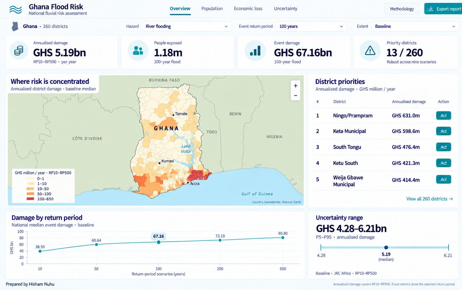
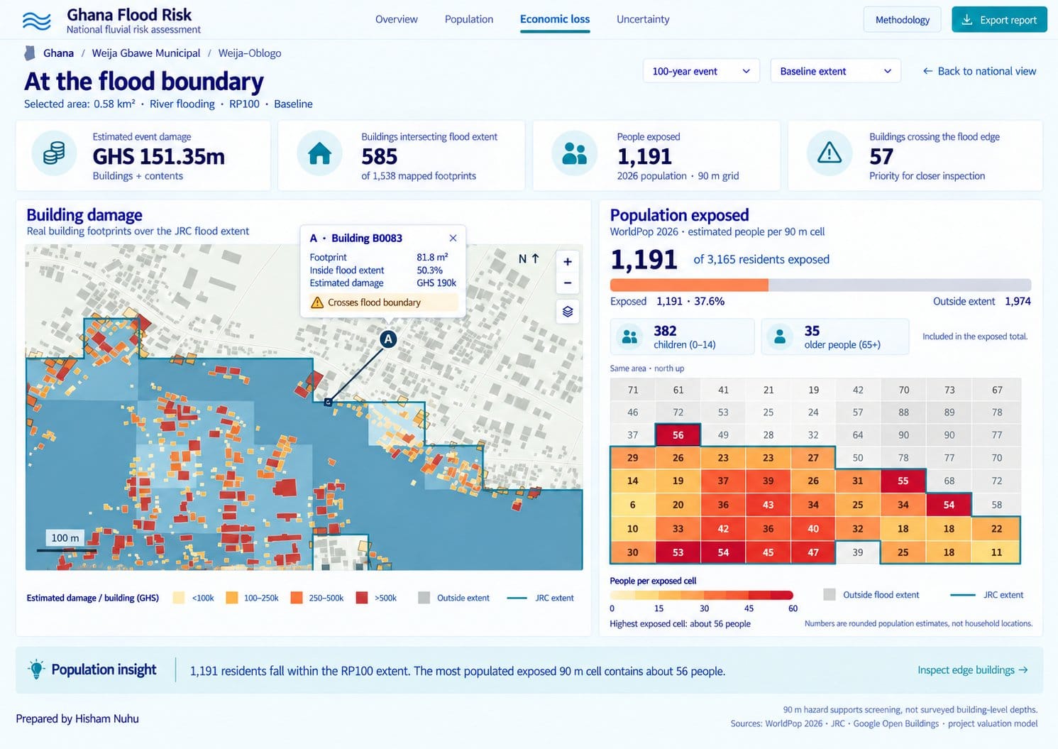
What a ministry could use: prototype decision-support dashboard views that go from 260 districts down to the buildings at the flood edge, with each figure beside its uncertainty and an action.

What the views do

A risk assessment helps only if a ministry or task team can act on it. I build decision-support tools that help governments observe, understand, plan and manage flood risk. My prototype dashboard views rank all 260 districts by modelled damage and people exposed. They show uncertainty beside every headline figure and give each district an action: Act, Investigate or Monitor. From there, a user would drill down to the individual buildings at the flood edge, where the national screen most needs checking on the ground. This serves Sendai Priority 1, understanding disaster risk, and Priority 2, giving institutions evidence they can govern with. The work has been presented for discussion with the World Bank.

Show the two prototype dashboard views: national and district
Fig. 9

Decision-support dashboard views (prototype): national overview and district drill-down

Prototype national overview dashboard view for Ghana’s river flood risk: scenario controls, four headline figures (GHS 5.19bn annualised damage, 1.18 million people exposed, GHS 67.16bn event damage, 13 of 260 priority districts), a district damage map, a table of the top five districts, a damage-by-return-period chart and an uncertainty range.
  1. Scenario controlsSwitch hazard, return period (10–500 years) and flood extent; every panel updates.
  2. Risk concentrates south-eastVolta delta and Greater Accra fringe: the top 5 districts hold 49% of national annualised damage.
  3. An action for every districtAct = in the top 20 under all nine model combinations (13 districts). Investigate 13, Monitor 234.
  4. Uncertainty in plain sightGHS 5.19bn a year (median), P5–P95 range GHS 4.28–6.21bn from Monte Carlo (Latin hypercube) sampling.

National view: modelled river-flood risk for 260 districts, with uncertainty and an action class for each (prototype views).

Select a pin or a note. These are prototype views of a dashboard, not a live service. The 90 m hazard supports screening, not surveyed building-level depths.

Sources

Sources: JRC, WorldPop 2026, Google Open Buildings and my valuation model; country boundaries Natural Earth.

How a ministry or task team would use the two views

How a ministry or task team would use the two views

StepViewQuestion it answersTypical use
1. National prioritisationNational viewWhere are modelled losses and exposed people largest, which districts stay priorities under every assumption, and how big is the uncertainty?Allocate assessment and project-preparation resources; agree a shortlist and a capacity threshold; check the economic ranking against people exposed.
2. District drill-downDistrict viewHow many buildings, how much asset value and how many people sit inside the modelled extent here, and how many are children or older people?Scope a local appraisal or terms of reference; target engagement, preparedness and early-warning outreach to the groups exposed.
3. The flood edgeDistrict view, building pop-upWhich buildings are only partly inside the extent, so the result depends on where the boundary falls?Build a field-verification list (floor levels, building use, flood marks); order a local survey or 2D modelling where it would change a decision.

What happens next

The national screen does not choose schemes. It decides where to look next, and each class leads to a different kind of work.

Act: 13 districts

Local appraisal, community engagement and a preparedness review.

Investigate: 13

Targeted evidence, such as terrain, building use and damage relationships, to settle whether the district belongs on the shortlist.

Monitor: 234

Reassessed as data and conditions change. Monitor does not mean safe.

Show the proposed 90-day scoping plan
Fig. 10

A proposed 90-day scoping plan

Days 1–30: agree ownership

Agree the government owner, the planning decision and the pilot criteria. Output: a partner agreement and an evidence inventory.

Success means an agreed decision, a responsible counterpart and a funded route to local appraisal. This is a scoping phase; detailed hydraulic design follows separately.

Sources

Proposal for discussion.

The proposed pilot

The proposed next step is a small, Ghana-led pilot that tests three different decision needs. The first is a district that stays a priority under every assumption: appraise options in their catchment context. The second is a district whose selection depends on the assumptions: test terrain, exposure and damage functions. The third is a district that ranks higher for people exposed than for asset value: add a social and critical-services criterion, for example adapting the UK Neighbourhood Flood Vulnerability Index, which combines susceptibility with the ability to prepare, respond and recover, and community support (Sayers and Partners, 2017).

The approach is informed by GFDRR and the World Bank’s Handbook for Livable and Resilient Cities: Integrating Hazard and Risk Information into Urban Planning (2025): agree ownership, refine priority locations, compare feasible measures, embed measures in spatial plans, then implement and update.

Limits of a national screen

Stated plainly, so the results are used for what they can support.

River flooding onlyNo surface-water or coastal flooding (the coast is screened separately), and no channels, defences or urban drainage beyond what the JRC maps contain.

Residential onlyHomes and contents. No infrastructure, agriculture or business losses, and every detected building is treated as residential.

Four more limits

Partial annual damageAnnual damage covers 1-in-10 to 1-in-500-year floods only. It is a comparable measure for ranking, not a national loss bill.

Transferred damage curvesNone of the three curves comes from Ghanaian damage records; they are tested as alternatives.

90 m screeningThe hazard grid supports national prioritisation, not building-level depths. A one-cell shift in the flood edge can multiply building counts more than six-fold.

No national building count in the extentThe final 90 m model reports damage and people; it does not report a national count of exposed buildings.

Next: extend the screen from river to sea How high can the sea reach on Ghana’s coast? How high tide, storm surge and waves can push the sea along 566 km of coast in 57 sections, with uncertainty ranges and a sea-level-rise screen. Understand, learn and adapt
Data and credits

Data: JRC Global River Flood Hazard Maps v2 (CC BY 4.0); Google Open Buildings v3; WorldPop 2026 (CC BY 4.0); VIIRS night-time lights (Earth Observation Group); Ghana Statistical Service 2021 Population and Housing Census; Copernicus Sentinel-1 via Global Flood Monitoring; boundaries OCHA/HDX COD-AB (Ghana Statistical Service).

Ghana results are modelled estimates from independent consultancy (2025–26; the river work was also my Oxford MSc dissertation), presented for discussion with the World Bank and now being shared with its Accra-based team. They are not official figures or priorities of the Government of Ghana or the World Bank.